Resistance between two points in a plane

I got well and truly nerd sniped the other day when my friend showed my this XKCD cartoon

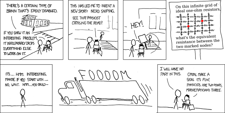Credit: XKCD.com

I never solved the "infinite grid of 1$\Omega$ resistors" problem because I had to involuntarily drop it when I realized it suggested another, more interesting, problem:

What is the resistance between two points on an infinite conductive sheet?

Imagine applying a voltage across two points separated by a distance $D$.  Now draw the contours of the voltage $V$ and also "lines of force" parallel to $\nabla V$.  This divides the plane into an enormous number of narrow strips.  The total resistance can be calculated by treating the areas between contour lines as resistors in series, and the strips between one contour and the next as resistors in parallel.

Take one strip of width $w$ and length $l$.  Its resistance is $cl/w$ for some constant $c$.  That means that if you scale up the entire picture by any factor, the strip's resistance does not change.  The consequence is that the total resistance between the two points does not change, and this is only possible if it is infinite!

Agh!  What went wrong?  It turns out we need to take into account the outline of each electrode.  The resistance between two points is only meaningful if you have a zero-diameter wires to attach to them, and zero-diameter wires have infinite resistance.  So, a better question is

What is the resistance $R_{\Omega}$ between two circles of radius $R$ with centres separated by $D$?

The answer is ... drum roll ...

$$
R_{\Omega} = \frac{c}{2\pi}ln\left(b + \sqrt{b^2-1}\right)
$$

where

$$
b = \frac{D^2}{2R^2}-1
$$

Let's see if we can work out why this is....  The scribblings below show my original working out, which I will summarize.

First off, let's see if we can get some inspiration.  My brilliant Physics teacher Mr Goddard taught me a model which works quite well: to determine the strength of a field you count the "lines of force" crossing each unit area of surface.  For spheres around a point charge the total area grows with $r^2$ but total number of "lines of force" remains the same, so the field strength is proportional to $1/r^2$.  Applying the same rule of thumb to a 2D situation we get a field strength proportional to $1/r$, which would imply a voltage proportional to minus its integral, namely $-ln(r)$.  This isn't terribly rigorous but it provides a guess we can come back to later on.

Next, let's see if we can derive a partial differential equation for the voltage $V$ outside of the footprints of the electrodes.  Here I'll use an observation I read in a great little book called "The Mathematical Mechanic": It turns out that in any network of resistors, when you apply a voltage across two points the remaining voltages settle to values that minimize the total power dissipation.  To prove this  imagine $N+1$ points connected by resistances $R_{ij}$, take $V_0$ and $V_N$ to be fixed, and then calculate the partial derivates $\partial/\partial V_k$ of the total power

$$
P = \frac{1}{2}\sum_{i,j}{\frac{(V_i-V_j)^2}{R_{ij}}}
$$

Next, substitute in the resistance law ($V_i-V_j=I_{ij}R_{ij}$) and Kirchoff's law ($\sum_j I_{ij} = 0$).  After doing that it turns out that all the partial derivatives are zero, and therefore the power is minimized!

In the continuous case of a sheet of homogeneous conductive material the total power is

$$
P = \frac{1}{c} \int \left| \nabla V \right|^2 dA
$$

and the condition that $P$ is minimized leads very quickly to a two dimensional Laplacian equation.

$$
\frac{\partial^2V}{\partial x^2} + \frac{\partial^2V}{\partial y^2} = 0
$$

Luckily for us, our initial guess of $ln(r)$ does indeed solve this p.d.e..  So does $ln(r_A)$ and $ln(r_B)$ where $r_A$ and $r_B$ are distances from arbitrary points $A$ and $B$.  And since the equation we are trying to solve is linear, $ln(r_A) - ln(r_B)$ is also a solution.

Contours of $ln(r_A) - ln(r_B)$

The next question we need to address is "what do the contours of $V = ln(r_A) - ln(r_B)$ look like?"  Let's choose $A$ and $B$ a distance $d$ apart

$$
\begin{align}
A &= (-\frac{d}{2},0) \\
B &= (+\frac{d}{2},0)
\end{align}
$$

Then, treating $V$ as constant and rearranging the equation we get the following contour for $+V/2$

$$
x^2 + y^2 - 2kx + k^2 = R^2
$$

where

$$
\begin{align}
k &= -\frac{d}{2}\left(\frac{1+e^V}{1-e^V}\right) \\
R^2 &= \frac{d^2}{4}\left(\left(\frac{1+e^V}{1-e^V}\right)^2-1\right) \\
\end{align}
$$

In other words, the contour is a circle around $(k,0)$ of radius $R$!  Likewise, the contour for $-V/2$ is a circle around $(-k,0)$ also of radius $R$.  We are getting close.  All we need to do now is calculate the current crossing one of the contour lines.  The simplest contour is $V=0$ and that's the vertical line $x=0$.

Consider an element $dx \times dy$ crossing the y-axis.  The voltage drop across it is $\partial_x Vdx$ and its resistance is $cdx/dy$ making the current across it equal to $\partial_x V dy/c$.  Integrating this is quite straightforward and results in a current of

$$
I = \frac{2\pi}{c}
$$

Giving a resistance of

$$
\begin{align}
R_{\Omega} &= \frac{(+V/2) - (-V/2)}{I} \\
&= \frac{Vc}{2\pi} \\
\end{align}
$$ 

The final step is to eliminate the arbitrary constant $V$ (which was used to find the contours for $\pm V/2$) and write it in terms of $D=2k$ (the distance that separates the centres of the two contour circles).  This is just straightforward algebraic manipulation and results in ... drum roll ...

$$
R_{\Omega} = \frac{c}{2\pi}ln\left(b + \sqrt{b^2-1}\right)
$$

where

$$
b = \frac{D^2}{2R^2}-1
$$ 

Now I can get back to whatever the hell it was I was thinking about before all this business....

Code for contour plot

import matplotlib.pyplot as plt
import numpy as np

X,Y = np.meshgrid(
    np.linspace(-2,2,1000),
    np.linspace(-2,2,1000))
Ra = ((X+1)**2 + Y**2)**.5
Rb = ((X-1)**2 + Y**2)**.5
V = np.log(Ra) - np.log(Rb)
plt.ion()
levels = np.linspace(-100,100,401)
plt.contour(X, Y, V,
            colors=['black'],
            levels=levels,
            linewidths=[1],
            linestyles=['solid'])
plt.gca().set_aspect('equal')
plt.axis('off')