- Get link
- Other Apps
Contents
- Intro
- Simple stratified model
- Alternative convection model
- Tropospheric temperature gradient
- Approach used in convection model
- Calculation of Radiative Forcing from CO₂ increase
- Calculation of Radiative Forcing from H₂O increase
- Calculation of zero-feedback ECS
- Effect of including feedbacks
- Effect of water vapour
- Effect of cloud cover change
- Effect of sea ice loss
- Calculation of ECS including feedbacks
- Limitations
- One more thing: Changes to Troposphere depth
Intro
The goal of this post is to see if we can come up with an estimate of Equilibrium Climate Sensitivity using a simple model in which the atmosphere is treated as well-mixed. By "simple" I mean that using the model will not require any advanced mathematics or computation, but will still be realistic enough to come up with an estimate within the likely range of 2.5 - 4.0°C predicted by the IPCC Assessment Report 6. I will try to take as little on trust as possible and show how the results are arrived at. In the process we will see where the famous log rule for Radiative Forcing comes from$^\dagger$.
Equilibrium Climate Sensitivity refers to the surface warming that would occur if CO₂ concentration doubled from the pre-industrial value of 280ppm to 560ppm over a short space of time, and then the climate system is allowed to "equilibriate". The word "equilibrium" presents a problem since a) it is possible that the system would not converge towards an equilibrium, and b) the time taken for this to happen may be too long for numerical models. To resolve these issues the definition is usually taken to include only short term responses - such as melting sea ice and heating of the ocean's shallow mixed layer - and not multi-century responses - such as melting land ice and heating of the ocean's depths. The precise set of what is and is not included is not agreed upon. For this reason it is instructive to perform the estimate oneself, as this is the only real way to understand the context, in particular what has been left out and what has been assumed.
Simple stratified model
In a previous post I described a simple one dimensional model of Earth's atmosphere. The atmosphere was modelled as stratified, that is layers could emit and absorb IR radiation but air could not move up and down. The model was then used to describe the greenhouse effect quantitatively, and to come up with an estimate of ECS. Although the assumption was unrealistic, and the model did not include any feedbacks at all, if did come up with a reasonable estimate of of 3.7°C.
Alternative convection model
But what if instead of a stratified atmosphere we modelled the atmosphere as well-mixed? The result is likely to be lower and we can use a simple analogy to see why. Imagine you are lying in bed under a blanket and someone adds a second blanket on top of that. After a while you will warm up. If more blankets are added gradually you'll keep getting hotter. However, if instead of allowing temperatures to settle, the blankets are rotated every few minutes, this allows a lot more heat to escape as warm blankets reach the top of the pile. And, as a result, your temperature at the bottom of the stack will be lower, and all the blankets will be the same temperature. From this argument we can expect that a convection model of the atmosphere that ignores feedbacks will come up with a lower estimate than 3.7°C.
Tropospheric temperature gradient
In the Troposphere, which makes up the majority of the atmosphere by mass, the air is indeed well-mixed. This does not result in a constant temperature with altitude as in the blanket analogy because pressure drops away as you go higher, and the ideal gas law $pV=nRT$ tells you that as a result either the temperature or air density must also drop. (In fact both do!) What is more or less constant though is the potential temperature $\theta$. This is defined as the temperature the air would obtain if a bubble of it was brought down to ground level adiabatically, that is without exchanging heat with the surrounding air. Air columns are only stable when the rate of change of potential temperature with altitude $d\theta/dz$ is positive. (If it's negative buoyancy causes neighbouring air pockets to swap places.) Heat is mostly injected at ground level which results in a constant shuffling of air packets until $d\theta/dz$ reaches zero.
Solving $d\theta/dz=0$ for $T(z)$ is relatively straightforward and results in the well known fact that temperature drops by 6.5C per km of altitude. The 1D stratified model in my earlier post does not predict temperatures dropping that fast, which is surprising as it suggests convection does not occur. However, in the real world heating is very uneven, with different amounts of insolation across days and nights, and across different latitudes. As a result the Troposphere does see vertical air movements in convection rolls known as Hadley cells.
Approach used in convection model
We shall assume a well-mixed atmosphere and adopt a different approach to the stratified model: instead of building a temperature vs altitude formula, we'll determine how the amount of IR spectrum blocked changes as CO₂ is added. This will enable us to infer a "radiative forcing" (an equivalent increase in solar power reaching each sqm of ground) per doubling of CO₂.
In the previous post I introduced $\tau$, a measure of optical thickness. $\tau$ is defined as $ln(F_{in}/F_{out})$, the log of the ratio of flux going into a material to the flux coming out. The nice thing about $\tau$ is that it is proportional to the amount of physical material facing the flux. Consequently, we may define the absorption cross section $\sigma$ as $\tau/n$, the optical thickness per molecule per square metre facing the radiative flux. Both $\tau$ and $\sigma$ depend on wavelength so we will write $\tau_\lambda$ and $\sigma_\lambda$ from here on. The following plot shows how $\sigma_\lambda$ varies for CO₂, and for water vapour, over a range of values of $\lambda$
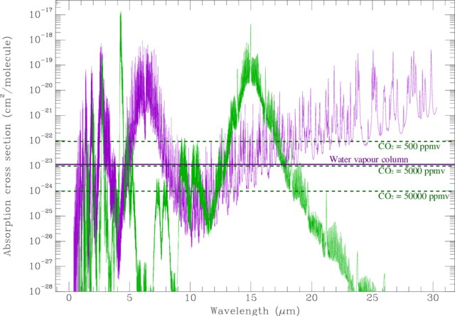 |
| Colin Goldblatt, Kevin J. Zahnle (2011) CC-BY-SA 3.0 |
Here's what this looks like when we scale up by the number of molecules in the atmosphere (in a vertical column with a $1m^2$ cross section), and convert the y-axis to a percentage of radiation blocked:
 |

A number of things are clear from these plots
- $\sigma_\lambda$ has a peak around 15$\mu m$ and this is the only peak that is relevant in the context of CO₂ blocking outgoing IR from Earth.
- At exactly this wavelength almost all outgoing IR radiation is already absorbed and, whilst adding more CO₂ will increase $\tau_\lambda$ it won't significantly alter the amount of IR blocked.
- However, the width of the wavelength interval around 15$\mu m$ that is effectively blocked will change as CO₂ is added.
- $log(\sigma_\lambda)$ is approximately linear between 12 and 15$\mu m$ and has a gradient of about +2/$\mu m$.
- $log(\sigma_\lambda)$ is approximately linear between between 15 and 21$\mu m$ and has a gradient of about -1/$\mu m$.
- In the region immediately to the right of the 15$\mu m$ CO₂ peak, water vapour is blocking all but about 20% of the outgoing IR.
- At 15$\mu m$, the outgoing IR has an spectral radiance of about 5.8 $Wm^{-2}/\mu m$ per steradian (a solid angle equivalent to $1/4\pi$ of a sphere).
From these observations we will calculate that the radiative forcing caused by increasing the CO₂ by a factor of $c/c_0$ is about $5.6ln(c/c_0)$ $Wm^{-2}$. This is very close to the oft quoted figure of $5.35ln(c/c_0)$ $Wm^{-2}$.
Our formula for RF means that doubling the CO₂ concentration is equivalent to about $3.9\ Wm^{-2}$ of additional radiation reaching Earth's surface. Later on we will scale this radiative forcing by what's known as a "climate sensitivity parameter" to obtain an estimate of ECS.
Calculation of Radiative Forcing from CO₂ increase
Let's see where the log rule for RF comes from!
Choose some high threshold $\tau_{thresh}$ for blocked outgoing IR. There will be two values $\lambda_1<15\mu m$ and $\lambda_2>15\mu m$ at which $\tau_\lambda$ crosses $\tau_{thresh}$. So we can say that, effectively, all IR in the ranges $[\lambda_1,15\mu m]$ and $[15\mu m,\lambda_2]$ are blocked. But since $\tau_\lambda=\sigma_\lambda n$, increasing $n$ (the number of CO₂ molecules per sqm) alters these ranges and therefore the amount of outgoing energy blocked.
Let's start with the first range $[\lambda_1,15\mu m]$. The equation $\tau_{\lambda_1} =\tau_{thresh}$ can be rewritten
n\sigma_{\lambda_1}=\tau_{thresh}
$$
Taking logs gives
log(n) + 2.0\lambda_1/\mu m + \text{const}_1 = \text{const}_2
$$
Solving for $\lambda_1$ and taking deltas gives
$$
\begin{align}
\Delta \lambda_1/\mu m&= -\frac{\Delta log(n)}{2.0}\\
&= -\frac{log(n/n_0)}{2.0}\\
\end{align}
$$
$$
\Delta P =- 2\pi \ u \Delta \lambda_1
$$$$
\Delta P = 2\pi \ u \frac{log(n/n_0)}{2.0}
$$$$
\Delta P = 2\pi \ u \frac{ln(c/c_0)}{2.0\ ln(10)}
$$
Calculation of zero-feedback ECS
 An increase in atmospheric CO₂ is converted into a Radiative Forcing in the same way we have described above. This is multiplied by an initial climate sensitivity parameter $\lambda_0$ which only takes into account the Stefan-Boltzman formula. According to our calculations $\text{toRF}(c/c_0) = 5.6\ ln(c/c_0)$ $Wm^{-2}$ and $\lambda_0 = 0.29\ KW^{-1}m^2$. Putting these together comes up with a feedback-free estimate for the surface heating $\Delta T$.
Effect of water vapour
Effect of cloud cover change
Effect of sea ice loss

It is reasonable to assume that at 2xCO₂ all sea ice will have
gone, given current trends. If we treat this loss of sea ice as an
additional forcing rather than a gain, working out the exact figure is
essentially just an integration task. This has been done
and the result is that the loss of all Arctic sea ice in summer is
equivalent to a global RF of $0.71\ Wm^{-2}$. Let's round this up to $1\
Wm^{-2}$ to include sea ice surrounding the Antarctic. This then adds approximately 25% to the
radiative forcing from a CO₂ doubling, and therefore also adds 25%
to an ECS that's calculated ignoring surface albedo changes.
$$
\begin{align}
\text{ECS} &= \lambda \times \text{total_RF} \\
&= \frac{\lambda_0 \times (RF_{2\times CO_2} + RF_{no\ ice})}{1-g} \\
&= \frac{\lambda_0 \times (RF_{2\times CO_2} + RF_{no\ ice})}{1-g_{wv}-g_{cl}} \\
&= \frac{0.29\times (3.9 + 1.0)}{1-0.4-0.2} \\
&= 3.6°C
\end{align}
$$
Limitations
\begin{align}
\Delta \lambda_1/\mu m&= -\frac{\Delta log(n)}{2.0}\\
&= -\frac{log(n/n_0)}{2.0}\\
\end{align}
$$
If we let $P$ be the outgoing IR power absorbed per sqm and $u$ the spectral radiance, then$^{\dagger_1}$
\Delta P =- 2\pi \ u \Delta \lambda_1
$$
or, in terms of n
\Delta P = 2\pi \ u \frac{log(n/n_0)}{2.0}
$$
Rewriting for concentration $c$ and using natural logs this becomes
\Delta P = 2\pi \ u \frac{ln(c/c_0)}{2.0\ ln(10)}
$$
Which is about $7.9 \ ln(c/c_0)$ $Wm^{-2}$. However, half of that blocked IR is simply returned to Earth because the atmosphere must re-radiate half up and half down to remain in energy balance$^{\dagger_2}$. So we're looking at more like $4.0\ ln(c/c_0)$ $Wm^{-2}$ of radiative forcing.
For wavelengths above 15$\mu m$ the gradient is half as large and so this ought to contribute double, i.e. around $8.0\ ln(c/c_0)$ $Wm^{-2}$. However, all but 20% of the outgoing IR is already blocked by water vapour, so the actual contribution is just $1.6\ ln(c/c_0)$ $Wm^{-2}$. This leaves us with a grand total of radiative forcing due to elevated CO₂ of
$$
\text{R.F.}=5.6\ ln(c/c_0)\ Wm^{-2}
$$
The coefficient in the literature is actually 5.35 but, of course, that used more sophisticated techniques and more accurate inputs. (I just eyeballed a couple of graphs for my inputs, and I assumed a constant spectral radiance over the relevant wavelengths!) But it's nice to know we can get in the ballpark using just street maths.
Calculation of Radiative Forcing from H₂O increase
We can find a similar formula for the effect of increasing the water vapour concentration. For the moment let's ignore the questions of what might cause such an increase and just do the calculation.
We need to simply repeat the calculations done above with CO₂, but with slightly different data. This time instead of just one peak there are two: one around 6.5 $\mu m$ and one around 30 $\mu m$. We can ignore everything to the left of the first peak and to the right of the second peak, because almost all IR in those ranges is already blocked (and because the intensity of outgoing IR is near zero at those wavelengths anyway).
The data for water vapour (obtained by eyeballing the graphs above) are that
- The gradient of $\sigma_\lambda$ to the right of the 6.5 $\mu m$ peak is about -1.5/$\mu m$
- The gradient of $\sigma_\lambda$ to the left of the 30 $\mu m$ peak is about +0.1/$\mu m$
- The spectral radiance of the outgoing IR is around 5 $Wm^{-2}/\mu m$ per steradian in both these regions
- About 80% of the outgoing IR is already blocked by CO₂ in the second region.
Repeating the calculation we did for CO₂ using these figures we obtain that increasing the concentration of water vapour is equivalent to an increase of $20\ ln(c/c_0)\ Wm^{-2}$ of solar radiation reaching the surface, to about 1 s.f.
We will use this later on when we consider feedbacks.
Calculation of zero-feedback ECS
So, how does this translate into an ECS? Well, to determine this we need to know the climate sensitivity parameter, also denoted $\lambda$. This is the change in equilibrium surface temperature per unit of radiative forcing. We can work it out very simply by taking the derivative of the Stefan-Boltzmann formula, and doing so returns a value of $\lambda =0.29\ KW^{-1}m^2$ $^{\dagger_3}$. Multiplying that by our RF estimate of 3.9 $Wm^{-2}$ gives an ECS of 1.1°C. This is much lower than the value of 3.7°C given by the stratified model (without feedbacks), as predicted by the blanket analogy.
Effect of including feedbacks
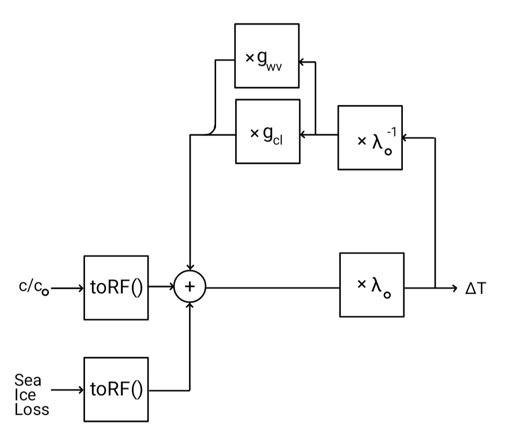
The standard model of feedbacks in climate science works as shown in the figure below

The next step is to adjust for feedbacks. An increase in surface temperature causes more water vapour to be held in the air, which can be treated as a radiative forcing of $g_{wv}\Delta T/\lambda_0$. Likewise the effect of changes to the clouds can be treated as a radiative forcing of $g_{cl}\Delta T/\lambda_0$, and the surface albedo changes caused by retreating sea ice can be treated as a radiative forcing of $g_{sa}\Delta T/\lambda_0$. These are considered the major feedbacks on the timescales we are considering but there are others too.
In principle the separate feedback gains can be summed to obtain an overall gain $g = g_{wv} + g_{cl} + g_{sa}$. The final climate sensitivity parameter is $\lambda = \lambda_0/(1-g)$ since $\Delta T= \text{toRF}(c/c_0) \lambda$ is the steady state solution to the loop.
Whilst this model works over short timescales, two things should be noted about $g$. The first is that a value of 1.0 represents a tipping point, and the second is that $g$ is not a constant. If summing together all the various feedback gains results in a value above 1.0 we should expect a chain reaction, but this won't continue forever. Instead $g$ will eventually return to a value below $1.0$, but in the process the climate will have switched to a new - warmer - state.
Effect of water vapour
To calculate $g_{wv}$ we need to calculate the radiative forcing caused by an increase in temperature of $\Delta T$.
For each extra degree, air holds 7% more water if we assume a constant relative humidity. This results in a RF of $20\ ln(1.07 \Delta T)$ $Wm^{-2}$ which is approximately $1.4\ \Delta T$ $Wm^{-2}K^{-1}$. We know this is equal to $g_{wv}\Delta T/\lambda_0$. Rearranging, and substituting in our previously calculated value of $\lambda_0$ gives $g_{wv} = 0.4$. This estimate is in line with estimates derived from computational models.
As previously mentioned, $g_{wv}$ is not constant. As temperatures rise the wavelength interval to the right of the main CO₂ peak - where IR can escape to space - will shrink to zero. When this happens, further increases in water vapour concentrations will have much less effect.
Effect of cloud cover change
Estimating the feedback caused by changes to cloud cover is really really hard and we are going to cheat by using a value calculated by others. We are going to use the results of a numerical study which estimates this to be 0.2. Putting this together with our estimate for $g_{wv}$ gives an overall $g$ of 0.6.
Effect of sea ice loss
In principle we could calculate a value for $g_{sa}$ by assuming a small $\Delta T$, determining how much sea ice is lost as a result, and calculating how much additional solar energy is captured to obtain a RF. In practice this is very difficult because of the geography of the Arctic and Antarctic make it hard to determine analytically exactly where the ice would be lost. There is however a simpler alternative if all we want is an ECS estimate:
Calculation of ECS including feedbacks
The final formula is therefore
\begin{align}
\text{ECS} &= \lambda \times \text{total_RF} \\
&= \frac{\lambda_0 \times (RF_{2\times CO_2} + RF_{no\ ice})}{1-g} \\
&= \frac{\lambda_0 \times (RF_{2\times CO_2} + RF_{no\ ice})}{1-g_{wv}-g_{cl}} \\
&= \frac{0.29\times (3.9 + 1.0)}{1-0.4-0.2} \\
&= 3.6°C
\end{align}
$$
The error bounds are obviously quite large and I invite you to play around and try alternative values for some of the estimated parameters that make up this calculation. I have done this myself and found that it is difficult to make the final figure stray outside the 2.5-4.0°C range that the IPCC have published in their AR6 report. Note that had we gone down the route of trying to calculate $g_{sa}$ then a value of 0.08 would have resulted in the same ECS figure.
Limitations
The major limitation of this, and in fact any, estimate of ECS is that it sidesteps the important issue of those feedbacks which alter the concentration of CO₂. When we emit CO₂ only half remains in the atmosphere. About a quarter is absorbed by plants and another quarter is absorbed by the oceans. These ratios may change over time, in particular warmer oceans may absorb CO₂ less readily. In addition to this, warmer surface temperatures lead to more forest fires, and melting permafrost, both of which release CO₂. If instead of asking what will happen if the concentration of CO₂ doubles we ask what will happen if we emit a given quantity of CO₂ we may get a much less certain answer.
Another thing missing from this analysis is the effect of other greenhouse gases, in particular methane. Some methane emissions can be considered a forcing, e.g. the methane released by a growing population of cattle, or the methane leaked during fossil fuel extraction. However, other methane emissions should be treated as feedbacks as they are caused by warming. Of particular concern is the methane released by melting permafrost. It is not fully understood to what extent melting permafrost will lead to CO₂ emissions and to what extent it will lead to the release of methane, a much more potent (if shorter lived) GHG. A consequence of this uncertainty is that this feedback is often not included in calculations, but that does not mean it is unimportant. It may be the difference between life and death.
When we take these limitations into account it becomes apparent that ECS estimates calculated in this way, while useful, cannot be relied upon to tell us "what will happen" if we emit this or that many tons of CO₂.
One more thing: Changes to Troposphere depth
You may wonder how it is possible for the surface temperature to change given that the temperature at the top of the atmosphere is fixed by the Stefan-Boltzmann law, and the temperature gradient is fixed at 6.5°C/km. The answer is that the Troposphere is growing! Above the Troposphere temperature starts climbing due to ozone molecules which absorb some of the incoming solar radiation. This prevents convection occurring above that altitude. (The boundary dividing convecting and non-convecting air is known as the Tropopause.) However, if surface temperatures rise, for whatever reason, then that boundary moves. And measurements have indeed shown that it has been rising at a rate of 50-60m per decade since the 1980s. Multiply this by 6.5°C/km (which is known as "the adiabatic lapse rate") and you find this growth in Troposphere depth roughly matches the increase in Surface Average Temperature (SAT) seen over the same period.
FOOTNOTES
- $\dagger$ That increasing the CO₂ concentration from $c_0$ to $c$
instantaneously is equivalent to increasing the solar radiation reaching
Earth's surface by $5.35\ ln(c/c_0)\ Wm^{-2}$.
- $\dagger_1$ The $2\pi$ is introduced here because $u(T,\lambda)$ refers to only one radian of solid angle (aka a steradian). There are $4\pi$ in a sphere, but only $2\pi$ of sky is visible from a single point on the surface. Clearly, the value of $n$ (the area density of CO₂ molecules) depends on the angle made with the ground. However, the final result for the radiative forcing will not depend directly on $n$, only the ratio $n/n_0$ and this is identical in all directions. This justifies the simplification we are making implicitly that all IR travels vertically upwards.
- $\dagger_2$ This is where we use the assumption that the atmospheric layers mix. In a model with no convection we cannot say that half is reradiated up and half down. This is because the reradiated energy may be absorbed by atmospheric layers above or below before reaching space or returning to the ground. The final ratio will only be 50:50 for IR initially absorbed at one specific altitude. However, if the air is constantly cycling through different altitudes, then whereever the IR is initially absorbed, the re-emissions will, on average, occur at half the optical depth of the Troposphere. At this location, half the energy emitted will ultimately make it to space and half to the ground.
- $\dagger_3$ The formula is normally written $P=\sigma T^4$ where $P$ is the area intensity of emitted radiation and $\sigma=5.67\times 10^{-8}Wm^{-2}K^{-4}$. However, if we are taking $P$ to be the total power coming from space and $T$ to be the temperature at the surface rather than the temperature seen from space, then we need to account for emissivity, the fact that some of the IR is returned by an atmosphere in energy balance. So, in place of the standard formula, we need to use $P=\epsilon\sigma T^4$. Setting $T=288K$ and $P=240 \ Wm^{-2}$ gives $\epsilon=0.62$. Substituting this into the derivative $dP=4\epsilon\sigma T^3dT$ and rearranging gives $dT=\lambda dP$ where $\lambda=0.29 \ KW^{-1}m^2$.
Comments
Post a Comment